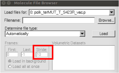
For the normal modes analysis, you need to have previously finished the cpptraj steps to create trajectory file for all the production steps. The topology file can be opened with vmd from the command line, but because the coordinate file is really large, it needs to be loaded in from the user interface. When loading in the data for the prmtop, set stride equal to 10 so that it only loads every 10 frames (see the image below).

$ vmd -prmtop vacuum.prmtop

Setting Stride

The Molecule File Browser for VMD. In the bottom left corner, there is a
box titled 'stride'. It should be set to 10.
Demonstration of where to set Stride to skip frames when loading the coordinate file.

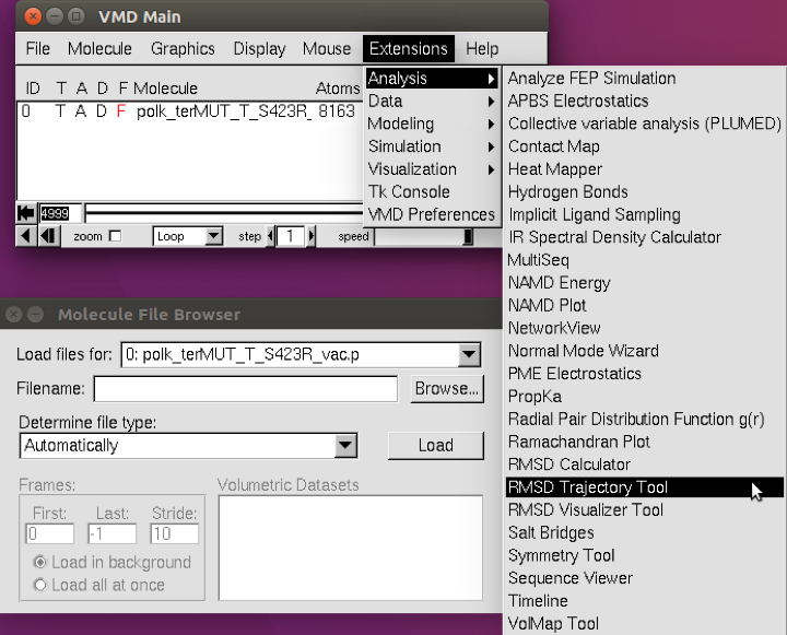
Once the trajectory files are loaded in, follow the VMD menu through Extensions → Analysis → RMSD Trajectory Tool (see below).

RMSD Analysis

Top left is the VMD Main Window. Extensions is highlighted, showing a
drop-down menu. From there, Analysis is highlighted, showing another drop-down.
Finally, RMSD Trajectory Tool is highlighted.
Location of RMSD Trajectory Tool.

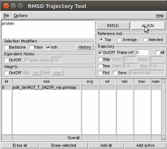
This brings up the menu (shown below) with several options. Click align.

RMSD Trajectory Tool

The RMSD trajectory tool. The top left says 'protein'. To the right of
that are two buttons: RMSD and Align. The cursor is over align.
The RMSD Trajectory Tool window, with the cursor over align.

After the structure is aligned, proceed to the Normal Mode Wizard. It can be found in the same menu as the RMSD Trajectory Tool, shown previously.

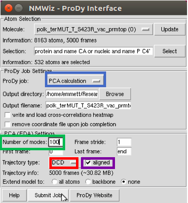
From the NMWiz menu, select ProDy Interface. This pulls up the ProDy window. Several things need to be changed in this interface, including setting the ProDy job to a PCA (Principle Component Analysis) calculation, changing the number of modes to 100 (it can analyze every mode, but the only important ones are the first few), changing the trajectory type to DCD, and clicking the aligned structure option. The aligned structure option is what was performed using the RMSD Trajectory Tool, and saves time in the normal mode calculation. After changing each of these, the job is ready to be submitted.

ProDy Interface

Top block is 'Atom Selection'. The first line is 'Molecule' with a
drop-down to select the PDB. The next line is information. Next is the
selection. The middle block is 'ProDy Job Settings.' The first is ProDy job.
Here, PCA calculation is outlined in blue. Next is the output directory. Next is
the output filename. There are two unchecked boxes, 'write and load
cross-correlations heatmap' and 'remove coordinates file upon job completion.'
The bottom block is 'PCA (EDA) Settings'. 'Number of modes: 100' is outlined in
green. Frame stride is 1, first frame is 0, last frame is end. The next line
contains the trajectory type. DCD is outlined in red, and the aligned box is
checked, outlined in purple. Next is trajectory info. None is selected for
extend model to. At the bottom are help, submit job, and ProDy Website buttons.
The ProDy Interface window. The necessary changes are emphasized with their corresponding colors: blue-ProDy job, green-number of modes, red-trajectory type, purple-aligned.

Once submitted, a new NMWiz window appears (see below). The mode that is being visualized appears in the upper left. From this window (and several successive windows), you can save the information for the normal nodes for further analysis and comparison. To do this, select Plot Mobility.

NMWiz Window

The NMWiz window. At the top left, 'Active mode: 1' is outlined in blue.
The next rows are scale options, then RMSD information, then selection. The
following row has 'Plot mobility' outlined in red. There are other blocks
of information, including actions with animation players.
The next NMWiz window, with the blue box corresponding to how to change between modes, and the red box corresponding to the Plot Mobility button.

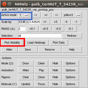
Plot Mobility brings up a plot (amazing!). The data from this plot need to be saved in a roundabout way. To start this process, go to File → Save as xmgrace. Title this file however you want, but recognize this will be done for more than 1 mode. Once saved, the Grace window will appear. In this window, follow Data → Export → ASCII. 
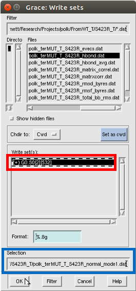
Yet another Grace window will appear, allowing you to save the data as a .dat file (see below). To actually save, first title the new file (under the selection box), and then click on the set in “Write Sets” that you want to save. Then, click OK. It won’t look like it did anything, so if you’re unsure if you clicked it, click OK again and it will ask if you want to overwrite the file.

xmgrace Window

The xmgrace window. The top line is the filter for listing files.
Next is a scroll block with files. What follows is an unchecked box with
'show hidden files.' The next block has change directory to the current
working directory. The next block is 'write sets' and the set of information
is highlighted and outlined in red. Then there is a format box. Next is 
the selection box, outlined in blue. Finally are the buttons 'OK', 'Filter',
'Cancel', and 'Help.'
The Grace window that allows you to save the normal mode data as a .dat file. In red is the set of data that should be selected and in blue is the save location.

Follow this process for the first 3 normal modes (1, 2, and 3).